Stochastic shape metrics without the agonizing pain

A no-math intuitive account of our method published in ICLR 2023.

Code for this post:

Code for methods in the paper:

Watch my 45min talk on shape metrics.

Neuroscience and machine learning experiments now produce datasets of several animals or networks performing the same task. Below are two matrices representing simultaneously recorded activities from neurons in two different networks.

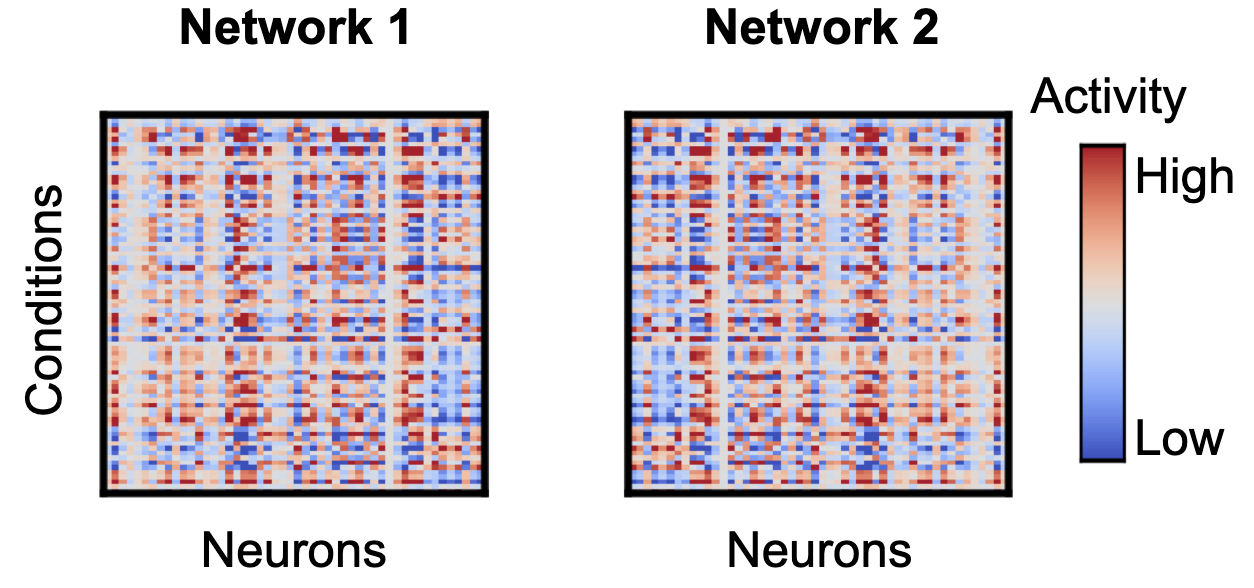
You can think of these as responses from two different animals, or two brain regions, or two deep net layers. Each column is a neuron and each row is the population response to a given stimulus condition. A fundamental question in neural representation learning & neuroscience is: Given multiple networks that were doing the same task, how related are their neural representations of the task? These two network matrices are high-dimensional, with the number of dimensions equal to the number of neurons, but for the sake of visualization, let’s assume responses each lie on some low 3D manifold of responses where each row of the matrix representing the population response to a condition is is plotted as a colored point in this space.

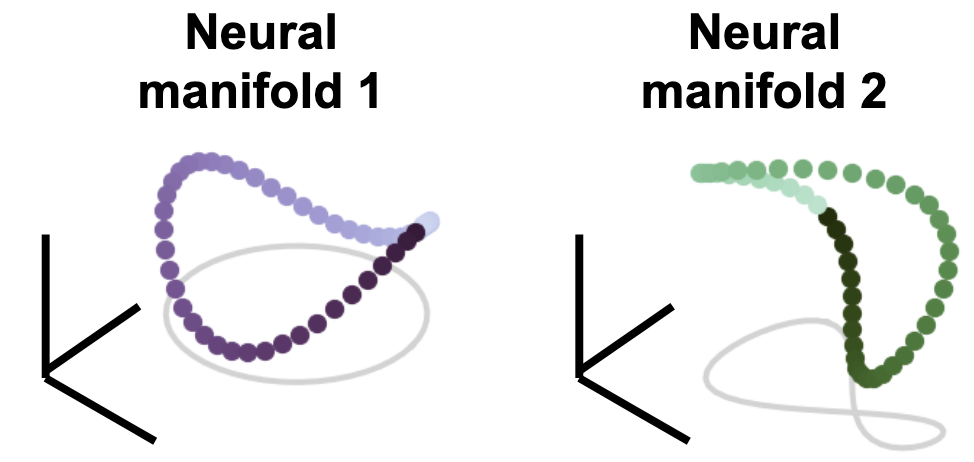
This manifold traces out a purple Pringles chip for network 1, and a green, slightly warped and rotated Pringles chip for network 2. How can we compare these representational geometric objects to each other, and how does that relationship correlate with the task? There have been many proposed methods to answer this question of network similarity, but I’m going to talk about a method and extensions to one that was proposed recently that draws from ideas from the field of statistical shape analysis (Williams et al. 2022).

Shape metrics on neural representations

We treat each joint response as a high-dimensional “shape” and wish to rigorously quantify notions of distance between these two shapes. The upshot is that the distance between these two geometric shapes should be independent given some group of nuisance transformations. For instance, the two manifolds above both look like Pringles chips, but are slightly warped and rotated from each other. So, even though the two manifolds are not exactly the same, in most cases, being a simple linear transform away from the other is not interesting. We are instead more interested in first aligning the representations, then analyzing the remaining differences. These ideas are used heavily in imaging registration, where we want to align two images of the same object (e.g. medical CT scans), but they are slightly rotated or translated.

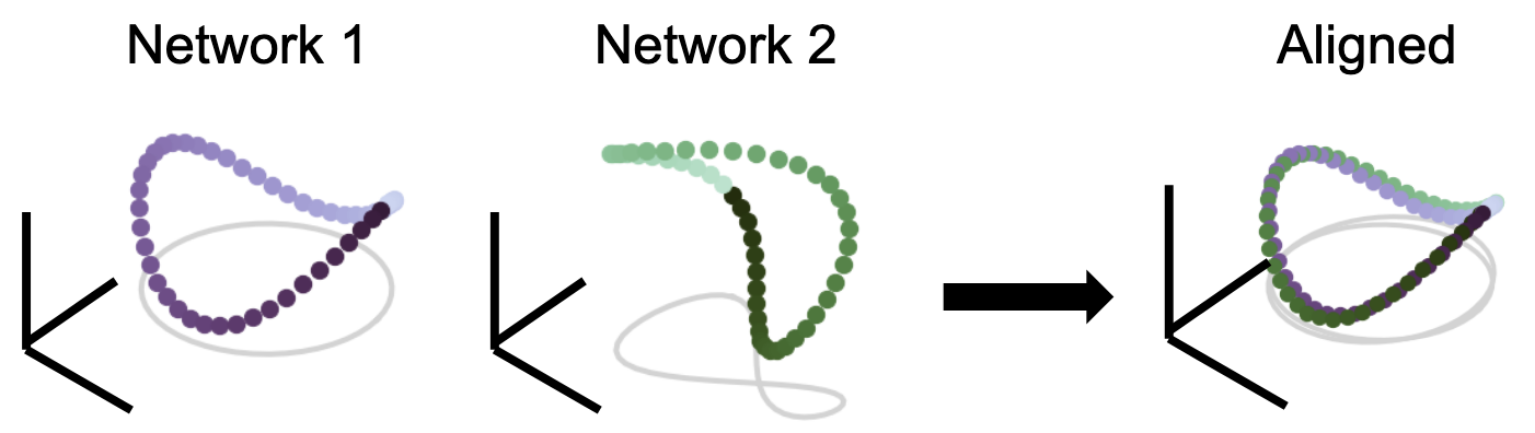
Given an allowable set of transformations (like a permutation, rotation/reflection, shifts, scaling), we should be able to first align the two networks, and whatever remaining difference is what we define as the distance between them. Indeed, how flexible or restrictive the chosen group of transformations is in itself an interesting hypothesis that the experimenter must decide on. Mathematically, this nuisance-transform invariant distance is a metric, which must obey these four properties:

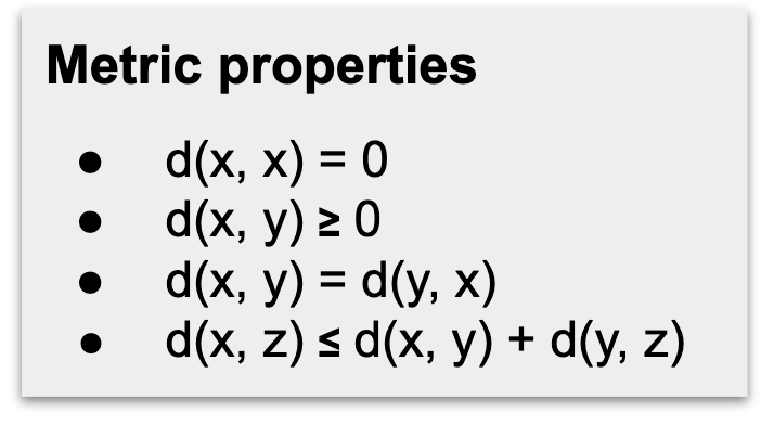
From top to bottom, these are: identity of indiscernibles, non-negativity, symmetry, and triangle inequality. These are the same properties that make Euclidean distance a metric. Because this is a bona fide metric, we can analyze pairwise distances between multiple networks simultaneously. This enables downstream clustering analysis and visualization with theoretical guarantees on correctness.

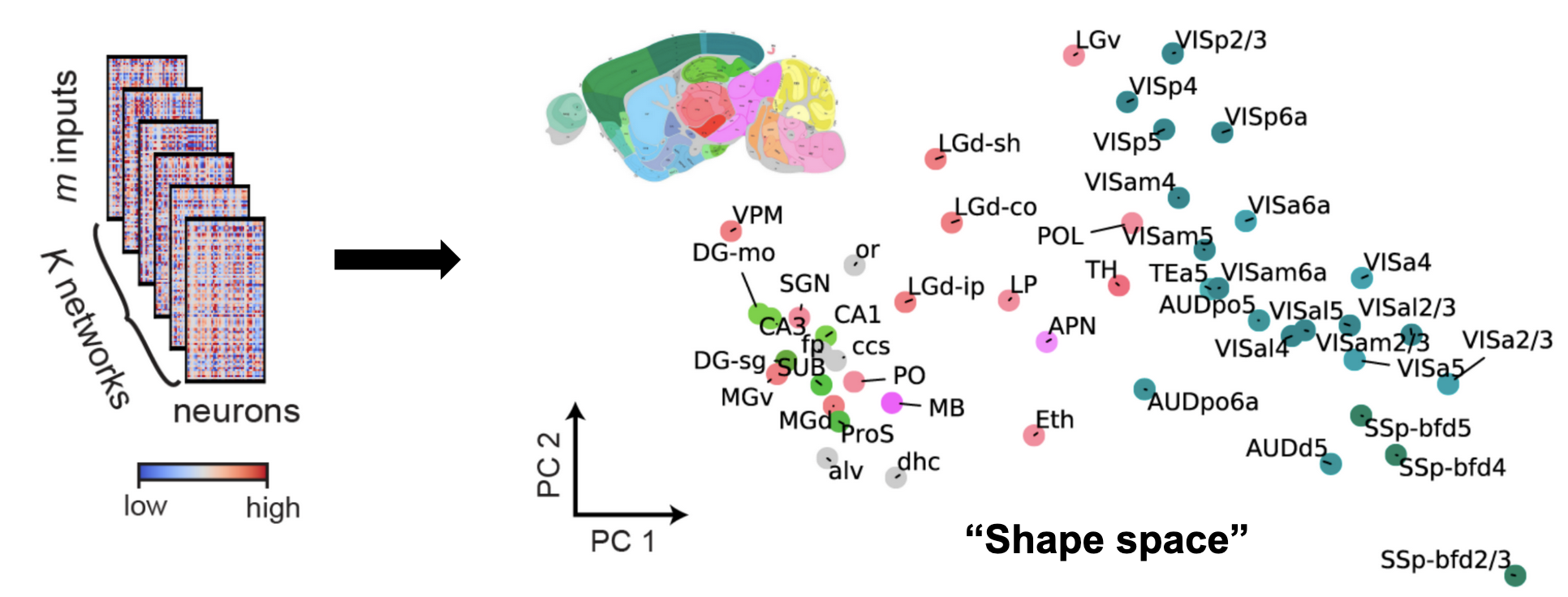
The plot above plot shows ~50 mouse brain areas from the Allen Brain Observatory. Analyzing their representational similarity with shape metrics allows us to plot all the networks in what we call “shape space”. The colors of each dot correspond to which brain area the network recording was from, and was only added after the fact. This shows that shape metrics provides an unsupervised way to discover functional similarity between different networks

Neural responses are noisy

The above-described shape metrics were derived for scenarios in which responses are deterministic; i.e. the same stimulus always elicits the same response. They can be applied to neural data where we have taken the conditional mean response across trials. But neural responses are stochastic! Imagine now that we show networks a stimulus (dark blue or cyan), producing a different response each time for each network.

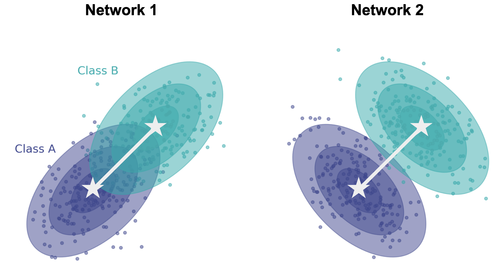
Note that the conditional means (white stars) are same in both networks, but the shape of the conditional distributions (ellipses) are very different. In neuroscience, these are referred to as “noise correlations”, and exist in all brain areas across all species. It’s therefore important for us to develop a way to compare how stimuli are encoded in different animals/networks not just by comparing the conditional means, but also the conditional noise. We need a notion of distance and an alignment procedure that takes into account noise in each response.

Dissimilarity between Gaussian representations

In the paper we describe ways of addressing stochasticity in comparing representational geometry, borrowing two ideas from the theory of optimal transport: Wasserstein distance and Energy distance. Here I’m only going to talk about Wasserstein distance.

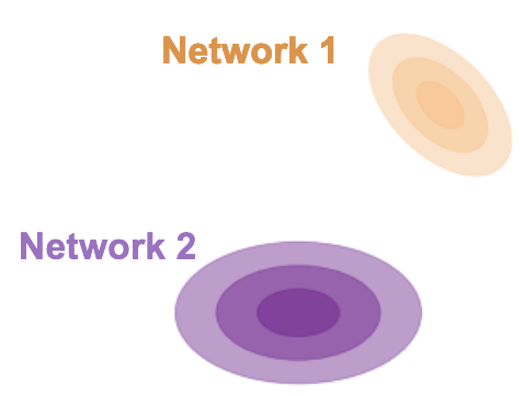
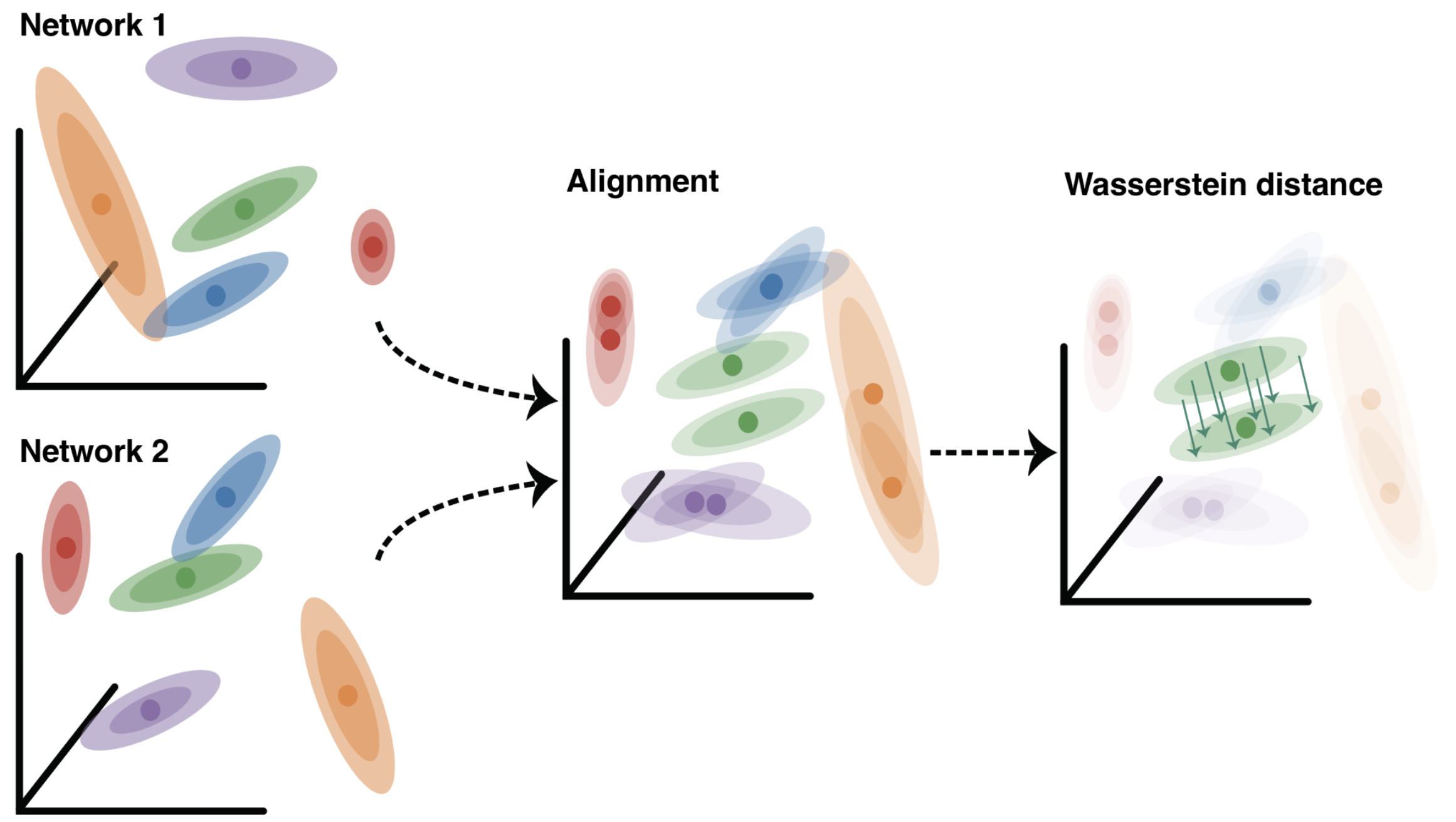
Consider two networks (purple and orange) responding to some condition with response mean and now with a covariance about that mean. If we model responses as Gaussian, then the 2-Wasserstein distance between them has the nice property of having an analytic solution which nicely decouples into two quantities familiar to experimentalists. The first term is simply difference between the network conditional means.

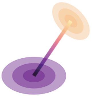
The 2nd is what’s known as the Bures metric, which quantifies the difference in orientation and scale of the covariance noise clouds.

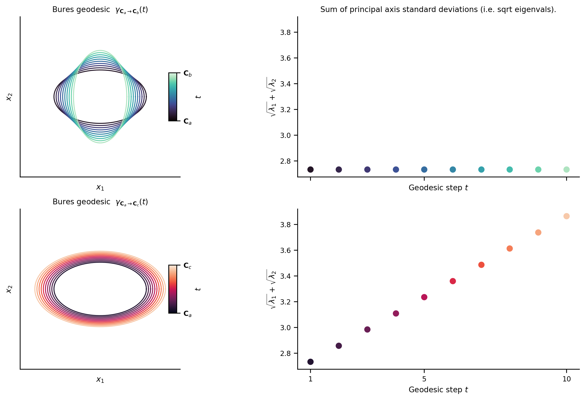
Geometrically, interpolating two covariances using the Bures metric traces out a path (a geodesic) between the two covariance clouds which linearly interpolates the sum of the principal axis standard deviations. The below plot shows the geodesic between covariance clouds \({\bf C}_a \rightarrow {\bf C}_b\) (90 degree rotation) and \({\bf C}_a \rightarrow {\bf C}_c\) (simple isotropic scaling). Note that the sum of principal axis standard deviations (i.e. sum of the square rooted eigenvalues) are linearly interpolated along the geodesic.

Intuitively, you can think of Wasserstein distance as the amount of work it takes to move and transform a pile of dirt that is shaped like the purple density to the orange one, or vice versa. Most importantly for us, Wasserstein distance is a metric, and therefore provides a natural stochastic extension to, and all the benefits of the deterministic shape metrics described above.

Stochastic shape metrics on neural representations

Equipped with the Wasserstein distance, we developed a procedure that can take two networks with stochastic responses and globally align them using a single transform, which now takes into account both their conditional mean & covariance structure. The remaining difference between them is quantified as Wasserstein distance distance between the two joint distributions.

Application: Variational Autoencoders

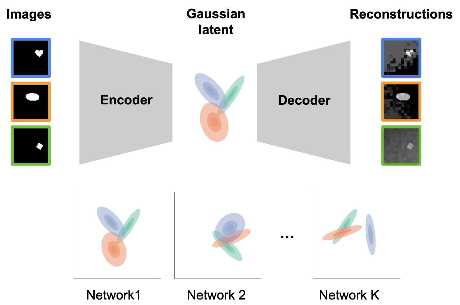
To demonstrate the utility and scalability of our stochastic shape metrics, we turn to variational autoencoders (VAEs). A VAE takes as input an image; after which, a neural network serves as a bottleneck to encode each input as a gaussian distribution. Another neural network then lifts out samples from these conditional densities to decode and reconstruct the input. These models are a perfect test-bed for our stochastic metric because the conditional responses are Gaussian by design, and so the Wasserstein distance is exact.

We used our method to compare 1800 different networks trained with different objectives and hyperparameters (Locatello et al. 2018). This distance matrix has about 1.6 million unique elements and would have taken ~10y of computation time if each pairwise distance was computed serially, but with some algorithm parallelization tricks, we were able to drop the compute time down from 10 years to a couple hours.

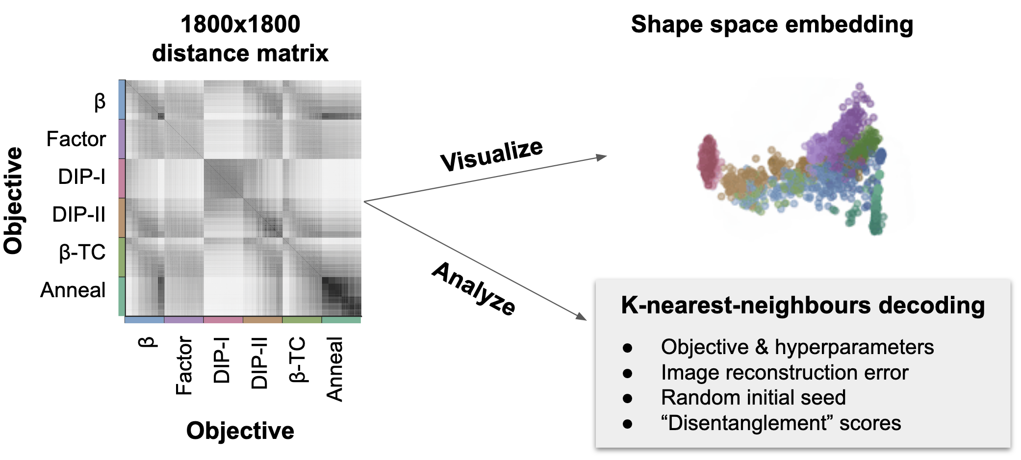
With this distance matrix, because our method defines a metric on stochastic representations, we can visualize and embed each network into shape space, and colour each network by its objective. We see that each colour clusters together as we might hope, and that our method reveals representational differences between networks trained with different objectives. Alternatively, we can use non-parametric K-nearest-neighbours analyses directly on the distance matrix. Doing this, we found that it’s possible to quantify and decode various parameters of interest such as the objective, how well each VAE reconstructed its inputs, how well the latents were “disentangled”, and even their random initialization seed!

Summary

Quantifying representational similarity is fundamental to neuroscience & ML. Shape metrics offer a principled way to compare responses of many networks. We develop shape metrics for stochastic neural responses. This method is highly scalable and can be used to compare thousands of networks simultaneously. These analyses can provide direct insight into how representational geometry relates experimental variables of interest (e.g. behaviour, task performance, etc.).