C++ neural networks from scratch – Pt 2. building an MLP
Building a trainable multilayer perceptron in pure C++.
![]()
MLP class
Now that we’ve built our matrix class and basic linear algebra functionality, let’s use it to build a multilayer perceptron (MLP).
We’ll first go through the class constructor, and then implement the forward() and backward() methods.
#pragma once
#include "matrix.h"
#include <random>
#include <utility>
#include <cassert>

using namespace lynalg; // matrix linalg lib from matrix.h
namespace nn {
template<typename T>
class MLP {
 public:
  std::vector<size_t> units_per_layer;
  std::vector<Matrix<T>> bias_vectors;
  std::vector<Matrix<T>> weight_matrices;
  std::vector<Matrix<T>> activations;

  float lr;

 ////////////////////////////////
 ///* Constructor goes here *////
 ////////////////////////////////

 ////////////////////////////////
 //* Forward method goes here *//
 ////////////////////////////////

 //////////////////////////////////
 //* Backward method goes here  *//
 /////////////////////////////////

};
}
Constructor
Time to make use of our matrix/linear algebra library from Part 1!
The MLP constructor will initialize a set of weights and biases for each layer, initialized to random Gaussian noise.
explicit MLP(std::vector<size_t> units_per_layer, float lr = .001f):
    units_per_layer(units_per_layer),
    weight_matrices(),
    bias_vectors(),
    activations(),
    lr(lr) {

  for (size_t i = 0; i < units_per_layer.size() - 1; ++i) {
    size_t in_channels{units_per_layer[i]};
    size_t out_channels{units_per_layer[i+1]};

    // initialize to random Gaussian
    auto W  = lynalg::mtx<T>::randn(out_channels, in_channels);
    weight_matrices.push_back(W);

    auto b  = lynalg::mtx<T>::randn(out_channels, 1);
    bias_vectors.push_back(b);

    activations.resize(units_per_layer.size());
  }
}
Forward pass
Each layer of the neural network will be of the form output <- sigmoid( Weight.matmul( input ) + bias ).
First, we can implement the sigmoid nonlinearity, which is pretty straightforward.
inline auto sigmoid(float x) {
  return 1.0f / (1 + exp(-x));
}
The forward pass consists of computing the activations at a given layer, saving it to activations, then pass it forward and use it as the input to the next layer.
auto forward(Matrix<T> x) {
  assert(get<0>(x.shape) == units_per_layer[0] && get<1>(x.shape));

  activations[0] = x;
  Matrix prev(x);
  for (int i = 0; i < units_per_layer.size() - 1; ++i) {

    Matrix y = weight_matrices[i].matmul(prev);
    y = y + bias_vectors[i];
    y = y.apply_function(sigmoid);
    activations[i+1] = y;
    prev = y;
  }
  return prev;
}
Backward pass
We’re going to need the derivative of a sigmoid wrt its inputs:
inline auto d_sigmoid(float x){
  return (x * (1 - x));
}
The backprop() class method we’ll make will take as input the target output.
We can apply the strategy described directly from Bishop Pattern Recognition and Machine Learning chapter 5.
It’s been covered in tons of other articles so I’m going to omit the details and only focus on the C++ implementation here.
This article has a good walk through for details.
void backprop(Matrix<T> target) {
  assert(get<0>(target.shape) == units_per_layer.back());

  // determine the simple error
  // error = target - output
  auto y = target;
  auto y_hat = activations.back();
  auto error = (target - y_hat);

  // backprop the error from output to input and step the weights
  for(int i = weight_matrices.size() - 1 ; i >= 0; --i) {
    //calculating errors for previous layer
    auto Wt = weight_matrices[i].T();
    auto prev_errors = Wt.matmul(error);

    // apply derivative of function evaluated at activations
    //backprop for biases
    auto d_outputs = activations[i+1].apply_function(d_sigmoid);
    auto gradients = error.multiply_elementwise(d_outputs);
    gradients = gradients.multiply_scalar(lr);

    // backprop for weights
    auto a_trans = activations[i].T();
    auto weight_gradients = gradients.matmul(a_trans);

    //adjust weights
    bias_vectors[i] = bias_vectors[i].add(gradients);
    weight_matrices[i] = weight_matrices[i].add(weight_gradients);
    error = prev_errors;
  }
}
Creating the neural net
Let’s write a helper function that will take as input the input and output dimensionality, and hidden layer specifications, and return an initialized model.
auto make_model(size_t in_channels,
                size_t out_channels,
                size_t hidden_units_per_layer,
                int hidden_layers,
                float lr) {
  std::vector<size_t> units_per_layer;

  units_per_layer.push_back(in_channels);

  for (int i = 0; i < hidden_layers; ++i)
    units_per_layer.push_back(hidden_units_per_layer);

  units_per_layer.push_back(out_channels);

  nn::MLP<float> model(units_per_layer, lr);
  return model;
}
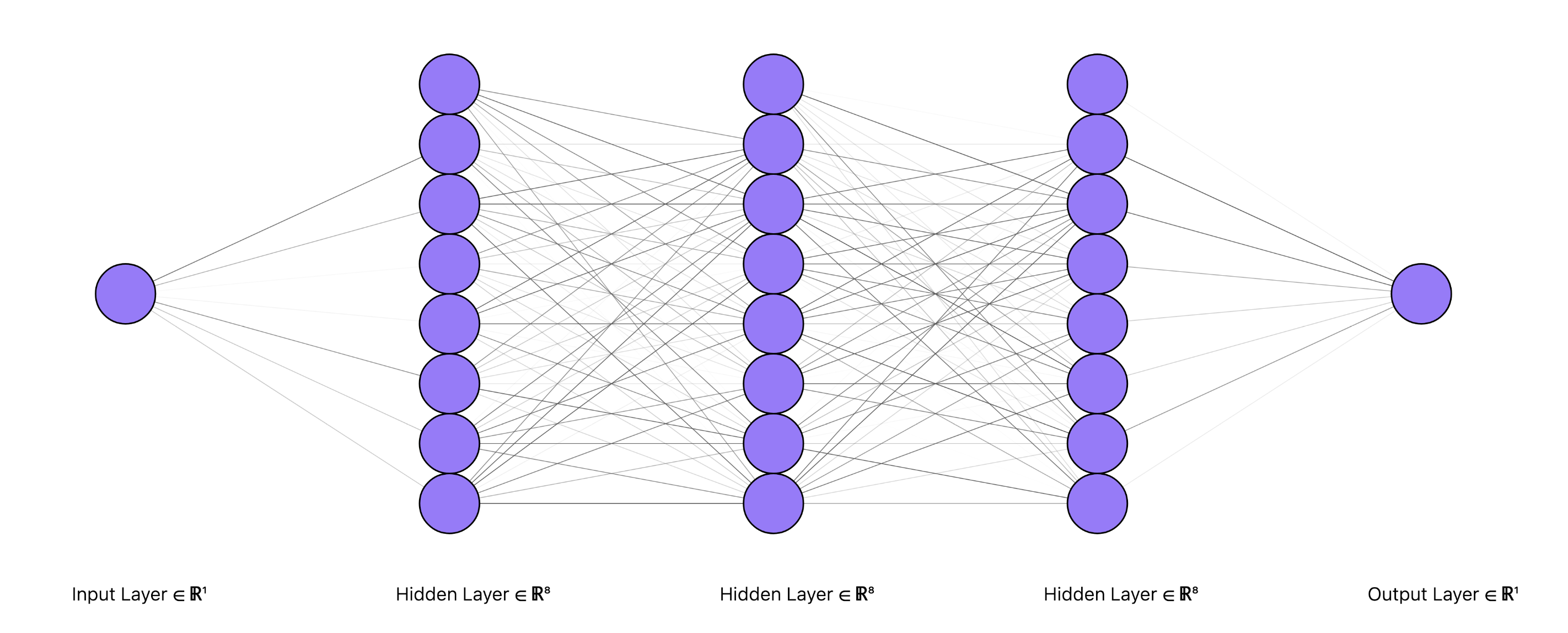
So if we want to initialize model with 1D input and output, and 3 hidden layers with 8 hidden units each, then we can just call our function like:
auto model = make_model(
  in_channels=1,
  out_channels=1,
  hidden_units_per_layer=8,
  hidden_layers=3,
  lr=.5f);
which would then yield a network architecture that looks like the above figure, with Gaussian random weights and biases.
Great – now that we’ve built a trainable multilayer perceptron on top of our bare-bones linear algebra library, it’s time to train it.