Stochastic gradient Markov chain Monte Carlo
PyTorch implementation and explanation of SGD MCMC sampling w/ Langevin or Hamiltonian dynamics.
![]()
![]()
The main takeaway of this post is that we can use gradient descent with injected stochasticity to sample an arbitrary target distribtion. Using familiar machinery we use to optimize (i.e. stochastic gradient descent; SGD), we can sample a density instead of just find its optima. I’ll show two implementations below: SGD sampling without momentum (Langevin Dynamics), and with momentum (Hamiltonian Dynamics).
The wiki page has more info and links to the papers outlining the procedures in detail
import torch
import tqdm
import numpy as np
from matplotlib import pyplot as plt
Let’s create a normal distribution to sample.
class NomalDist:
    def __init__(self, mu, sigma):
        self.d = len(mu)
        self.mu = mu
        self.sigma = sigma
        self.sigma_inv = torch.inverse(self.sigma)
        self.sigma_cho = torch.cholesky(sigma)

    def loss(self, x):
        """Quantity to be optimized later (neg log density of distribution in this case)"""
        return (x - self.mu).T @ (self.sigma_inv @ (x - self.mu))

    def sample(self, n_samples):
        """Helper to return samples of distribution"""
        z = torch.randn((n_samples, self.d))
        samples = (self.sigma_cho @ z.T).T
        samples += self.mu
        return samples
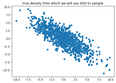
plt.figure(figsize=(7, 5))

mu = torch.zeros(2)
sigma = torch.tensor([[10, -8.],
                      [-8., 10]])
dist = NomalDist(mu, sigma)

original_samples = dist.sample(1000)
plt.plot(original_samples[:, 0],
         original_samples[:, 1], 'C0o')
plt.title('true density from which we will use SGD to sample')
Stochastic gradient Langevin dynamics
The idea is to inject noise into SGD as we’re optimizing, and that will better allow us to sample high-probability regions of the density. The only thing we need is some definition of loss (defined above as negative log density), and a black-box method w/ params $\theta$ over which to optimize. We can define the update equation for params to sample, $\theta$ at time $t$.
\(\theta_t \leftarrow \theta_t - \frac \epsilon 2 \cdot \nabla_{\theta} \log p(\theta_t \vert D) + \eta_t,\) \(\eta_t \sim \mathcal N(0, \epsilon).\)
\(\eta\), eta is our stochastic noise that we are adding. The first two terms on the RHS of the first eq are just standard gradient descent with step size $\epsilon$ and no momentum. If we include momentum, then this would be equivalent to stochastic MCMC w/ Hamiltonian dynamics instead of Langevin Dynamics.
But how do we inject noise? We use the fact that \(\frac{d}{d\theta} \eta\theta = \eta\), i.e. the derivative of a linear function of \(\theta\) is just a constant. So we first multiply noise with the parameters_, add this new (noise\(\times\)param) term to the existing parameters, and then differentiate the sum (call backward()).
class SGLD:

    def __init__(self, params, eta, log_density):
        """
        Stochastic gradilog_densityent monte carlo sampler via Langevin Dynamics
        Parameters
        ----------
        eta: float
            learning rate param
        log_density: function computing log_density (loss) for given sample and batch of data.
        """
        self.eta = eta
        self.log_density = log_density
        self.optimizer = torch.optim.SGD(params, lr=1, momentum=0.)  # momentum is set to zero

    def _noise(self, params):
        """We are adding param+noise to each param."""
        std = np.sqrt(2 * self.eta)
        loss = 0.
        for param in params:
            noise = torch.randn_like(param) * std
            loss += (noise * param).sum()
        return loss

    def sample(self, params):
        self.optimizer.zero_grad()
        loss = self.log_density(params) * self.eta
        loss += self._noise(params)  # add noise*param before calling backward!
        loss.backward()  # let autograd do its thing
        self.optimizer.step()
        return params
The _noise() method is where we implement the gradient noise trick described above.
Create a starting point before running the sampler.
x = torch.tensor([-10., 0], requires_grad=True)
sgld = SGLD([x], eta=1e-1, log_density=dist.loss)
samples = []

for epoch in tqdm.tqdm(range(10000)):
    x = sgld.sample(x)
    samples.append(x.data.clone().detach().T)

samples = np.vstack(samples)
100%|██████████| 10000/10000 [00:02<00:00, 3610.21it/s]
plt.plot(original_samples[:, 0], original_samples[:, 1], 'C0o', label='true density samples')
plt.plot(samples[:, 0], samples[:, 1], C1, label='samples')
plt.legend()
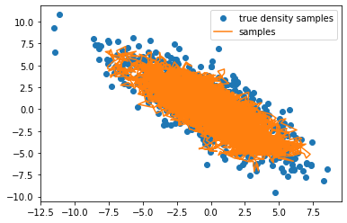
Looks great – it’s sampled the distribution pretty thoroughly!
Now let’s add momentum and build a Hamiltonian stochastic gradient MCMC sampler.
It’s pretty much the same idea as before but with non-zero momentum parameter in optim.SGD().
class SGHMC:

    def __init__(self, params, alpha, eta, log_density):
        """
        Stochastic Gradient Monte Carlo sampler WITH momentum
        This is Hamiltonian Monte Carlo.

        Paramters
        ---------
        alpha: momentum param
        eta: learning rate
        log_density: loss function for given sample/batch of data
        """
        self.alpha = alpha
        self.eta = eta
        self.log_density = log_density
        self.optimizer = torch.optim.SGD(params, lr=1, momentum=(1 - self.alpha))

    def _noise(self, params):
        std = np.sqrt(2 * self.alpha * self.eta)
        loss = 0.
        for param in params:
            noise = torch.randn_like(param) * std
            loss += (noise * param).sum()
        return loss

    def sample(self, params):
        self.optimizer.zero_grad()
        loss = self.log_density(params) * self.eta
        loss += self._noise(params)
        loss.backward()
        self.optimizer.step()
        return params
x = torch.tensor([0, 0.], requires_grad=True)
sghmc = SGHMC([x], alpha=0.001, eta=1e-4, log_density=dist.loss)
samples = []

for epoch in tqdm.tqdm(range(100000)):
    x = sghmc.sample(x)
    samples.append(x.detach().clone().T)

samples = np.vstack(samples)
100%|██████████| 100000/100000 [00:27<00:00, 3595.87it/s]
plt.plot(original_samples[:, 0], original_samples[:, 1], 'C0o', label='true density samples')
plt.plot(samples[:, 0], samples[:, 1], "C1-", label='samples')
plt.legend()
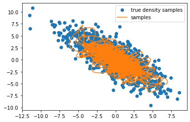
You can see the effect momentum has. Doesn’t look nice here (I had to take 10x more samples than with Langevin sampling), but for non-trivial density (e.g. banana-shape), it might help you traverse the density more effectively.