Nonlinear neural data dimensionality reduction with PI-VAE
Poisson-Identifiable Variational Autoencoder w/ PyTorch implementation.
![]()
![]()
Dimensionality reduction for neural data
Dimensionality reduction is a well-known concept to neuroscientists who deal with multi-neuron datasets. The central idea is that, despite having recorded from hundreds (nowadays even thousands) of neurons during an experiment, the underlying activity of those neurons is in fact low-dimensional. In other words, only a few dimensions are necessary to faithfully explain your data. These dimensions/axes are latent (meaning they are concealed), and exactly which select dimensions are necessary to explain your data is usually not known.
Imagine you ran some experiment where you show different one of five different colours to an animal while recording neural responses.
You recorded 100 neurons’ firing rates in a single experimental trial and store them as some 100-dimensional vector x.
You repeated this for N trials during your experiment and each of the five colours were presented for N/5 trials.
Latent variable models
It’s useful to approach the problem from a data generation point of view.
For each trial, we can model our data as some unobserved (latent) low-dimensional vector z being mapped through some function parameterized by \(\Theta_x\) up to a 100-dimensional vector of observed neural activities, x.
Using the useful notation of probabilistic graphical models (left plate model below) x and z are both random variables (denoted by circles below), but x is observed (shaded circle) while z is not (empty circle).
The observed vector x depends on both z and the mapping from z to x, parameterized by \(\Theta_x\), so arrows point from z and \(\Theta_x\) to x.
Our data comprises N total trials, with a different x and z on each trial; this is captured by placing the random variables on a rectangular plate, with N denoting the number of repetitions in the dataset.
Importantly, the parameters \(\Theta_x\) are off of the plate, because we assume the transformation from x -> z doesn’t change from trial-to-trial.
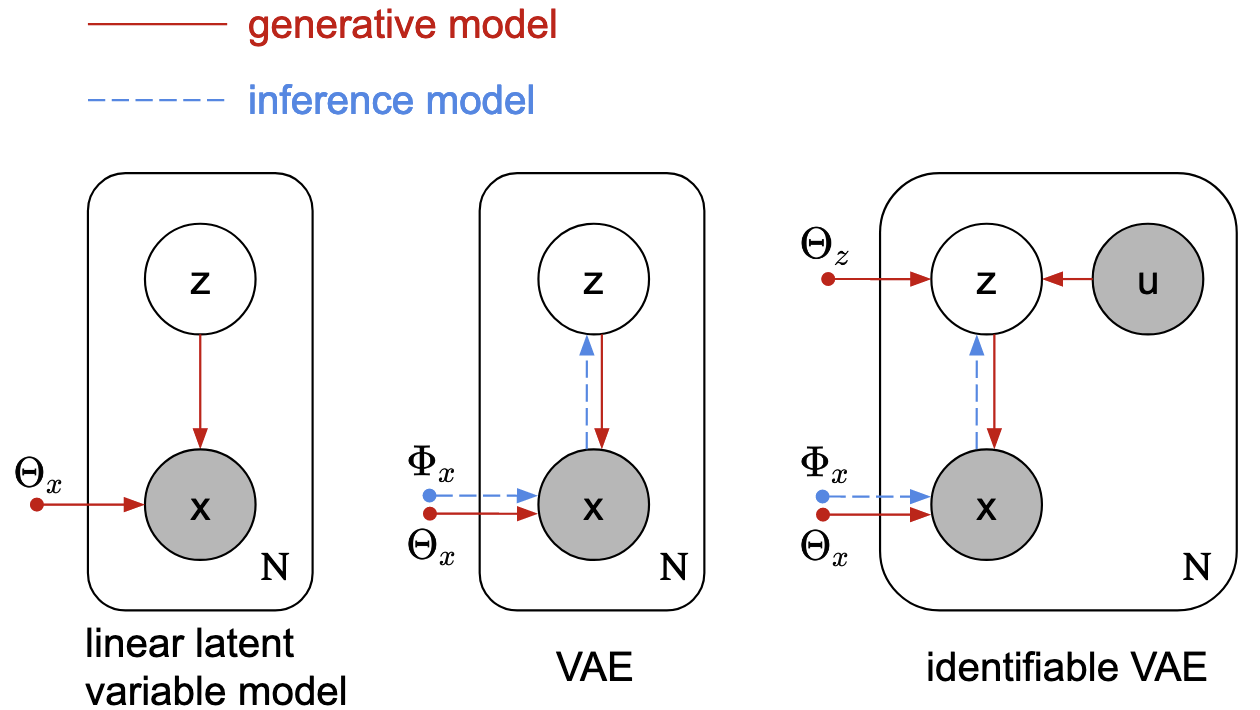 (This fig was made by myself and a couple others in the lab. We’re working on a project to extend ideas of the right-most model, which I will go into below.)
The model described thus far is very general.
For example, if the mapping z -> x is parameterized by \(\Theta_x\), and is linear, then we would be describing our data using linear dimensionality reduction methods.
Our choice of probability distribution used to model the latent variable z is also important: e.g. if z normally distributed with isotropic covariance, then we would be doing principal components analysis (PCA); or if z where normally distributed with diagonal covariance, then we would be doing factor analysis.
Nonlinear latent variable models and non-identifiability
PCA is one of the first dimensionality reduction techniques that people learn (although it’s usually introduced as a variance-maximization method and not than probabilistically as I did here), and is probably the most commonly used. Unfortunately, neural data is complex and linear dimensionality reduction methods are typically insufficient in fully describing data.
People have recently turned to more powerful nonlinear models, like variational autoencoders (VAEs; middle plate model above), to discover latent structure in their data. However, the increased expressiveness of nonlinear methods comes at the cost of identifiability, meaning that infinitely many (nontrivial) configurations of the latent space can explain the observed data equally well. This is a major issue if our ultimate goal is scientific discovery and interpretability of our data.
The Poisson Identifiable VAE
A recent paper proved that not all hope is lost, and that we actually can achieve identifiability in VAEs. The main takeaway is: if we condition our latent variable z on an another random variable, u, then we gain identifiability of the latent variable.
A direct application of this idea to neural data was used in a NeurIPS paper by Zhou and Wei (2020), the Poisson Identifiable VAE (PI-VAE).
The model is called Poisson Identifiable because the observed variable x is modelled as Poisson-distributed, as is typical for neural spiking data.
Using our 5-colour experiment described earlier as an example, in addition to our 100-dimensional observed x and low-dimensional z, we now introduce an observed u variable (right plate model in the figure above).
Intuitively, if we encode the colour directly into u, then our latent z|u becomes fully identifiable (up to trivial transformations like axis permutations and scalings).
The usual posterior found in vanilla VAEs, \(q(z|x)\), is replaced by \(q(z|x,u)\), and this posterior is further decomposed as the product
\[q(z|x,u) \propto q(z|x)p(z|u),\]where \(p(z|u)\) is a conditonal prior on \(z\).
In vanilla VAEs, \(p(z)\) is typically an isotropic Gaussian, meaning all points, regardless of trial colour, will be drawn from a single normal distribution in the latent space.
By conditioning z|u, \(p(z|u)\), is now a mixture of Gaussians, and allows each colour to be dissociable/disentangled in the latent space.
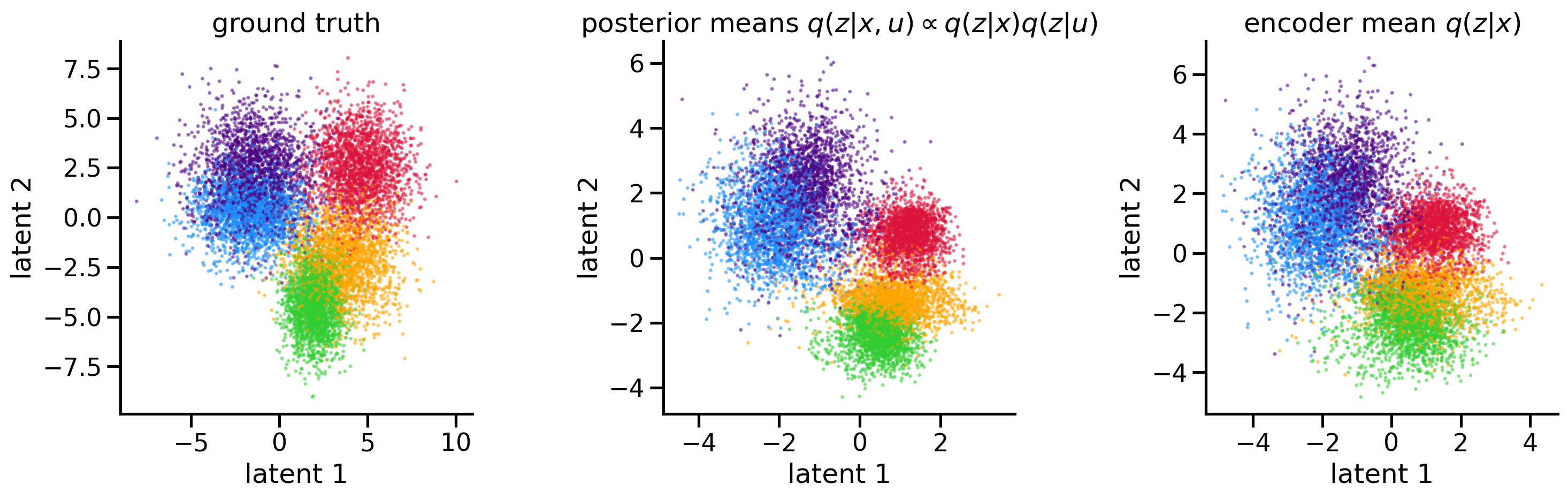
I re-implemented the PI-VAE model in PyTorch and recreated their Figure 2 in the spirit of our hypothetical colour experiment.
(There’s a lot of code so I didn’t include it here but the interactive code can be found at the top of the page.)
First, I generated a true 2D latent z as a mixture of Gaussians (one for each colour), and plotted them below on the left; there are N datapoints total representing N trials.
I nonlinearly mapped each 2D z to a 100D poisson-distributed x.
After training the PI-VAE on N trials of 100D data, with each trial having an associated observed u, the model successfully extracted the original latents.
There are some choices in the PI-VAE model that I don’t necessarily agree with (like their decoder architecture), but overall I like the model. In general I think idea of provable identifiability for neural data analysis is powerful, and is worth pursuing further + extending.