Batch and instance whitening

This short post will cover graphical intuition and PyTorch code for two different kinds of whitening: batch and instance.

Intro

Whitening is a fundamental concept in statistics, and turns up very often in machine learning. E.g. it can make it a lot easier to compare/transform distributions of activations like in style transfer. Whitening responses can also serve to efficiently propagate signal down a cascade of neural net layers.

The whitening operation is simple to understand geometrically: if your distribution is elliptical like a correlated Gaussian, then it turns it spherical. In 2D this means it turns an ellipse into a circle. Computing it is also relatively simple: you whiten your data with respect to statistics (covariance) of the data. The tricky part is to decide which aspect of your data you should be whitening.

Generating and plotting neural net activations

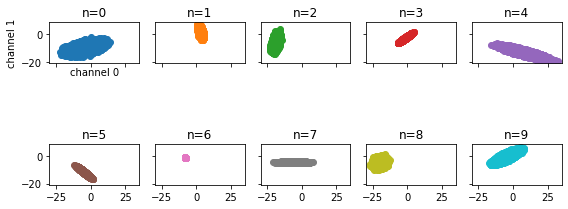
Let’s simulate activations of two convolutional filters (channels) to 10 images in a batch. The tensor of activations is Size([n=10, c=2, h=256, w=256]). If we collapse the spatial dims, we can plot the two filter responses against each other and see how they’re correlated and distributed.

Each entry in the batch dimension n=0:9 is referred to as an instance. Data is created by randomly colouring the channels’ responses in each instance (local covariances), then random means are added to the data, then the entire batch is randomly coloured according to some (global covariance).

"""Helper methods are in code repo linked above"""
def get_activations():
    """Creates 2D Gaussian distributed activations, with means distributed randomly."""
    a = torch.randn(shape)
    # colour locals
    a = torch.stack([colorize(flatten_space(r)) for r in a])
    a = unflatten_space(a)
    a += torch.randn((n,c,1,1)) * 10  # random means
    # colour global
    a = unflatten_batch_and_space(colorize(flatten_batch_and_space(a)))
    return a

activations = get_activations()

print("shape -- nbatch, nchans, height, width: ")
print(activations.shape)

output:
shape -- nbatch, nchans, height, width: 
torch.Size([10, 2, 512, 512])

Instance responses (local responses) look like ellipses:

# local responses
feature_scatter(activations)  # plotting code in repository

And globally, on one plot they look negatively correlated:

# plot all on single plot, but w/ same colours
feature_scatter(activations, nrows=1, ncols=1)

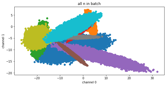
Each instance with local instance covariance is plotted in a different colour. The global batch covariance of the data looks to be negatively correlated.

Batch vs instance whitening

Here is the main takeaway and intuition:

Batch whitening: whiten all channels using each instance (image) in the batch.

Instance whitening: whiten all channels using single instance in the batch.

Batch whitening

The logic for batch whitening is simple: first, turn the 4D Size([n, c, h, w]) tensor into a 2D Size([n, (c*h*w)]) tensor. We then compute its covariance, and corresponding Size([c, c]) whitening matrix and apply it to the de-meaned data. Finally, we add back the mean and reshape the data back to Size([n, c, h, w]).

(This code could be greatly optimized but this way is easiest to understand.)

def batch_whiten(batch_feature_map):
    """zca whiten each feature using stats across all images in batch"""
    y = flatten_batch_and_space(batch_feature_map)
    y, mu = demean(y)
    N = y.shape[-1]
    cov = y @ y.T / (N - 1)
    # form whitening zca matrix:
    u, lambduh, _ = torch.svd(cov)
    lambduh_inv_sqrt = torch.diag(lambduh**(-.5))
    zca_whitener = u @ lambduh_inv_sqrt @ u.T
    z = zca_whitener @ y
    return unflatten_batch_and_space(mu + z)

batch_whitened = flatten_batch_and_space(batch_whiten(activations))
feature_scatter(batch_whiten(activations), nrows=1, ncols=1)

demean_batch_whitened, _ = demean(batch_whitened)
print('Global cov should be close to identity: \n',
      demean_batch_whitened @ demean_batch_whitened.T / batch_whitened.shape[1])

output:
Global cov should be close to identity: 
 tensor([[1.0000e+00, 2.8164e-07],
        [2.8164e-07, 1.0000e+00]])

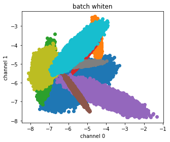
The data has been rotated and scaled, and now has identity covariance in aggregate. Clearly despite it having identity covariance it doesn’t look like a circular Gaussian at all. This is cheaper to compute relative to instance whitening, and the signal is more tame to work with now tha it’s been transformed.

Instance whitening

The logic here is similar to before. We start with a 4D Size([n, c, h, w]) tensor, and reshape it now to a 3D (not 2D) Size([n, c, (h*w)]) tensor. Then, we compute the covariance and whitening transform for each instance in the batch dimension. So there are now n tensors each with size Size([c, (h*w)]) with which to compute covariances and whitening transforms. These Size([c, c]) covariances describe the local covariances (coloured ellipses) shown above.

def instance_whiten(batch_feature_map):
    """zca whiten each feature map within individual image in batch"""
    y = flatten_space(batch_feature_map)
    y, mu = demean(y)
    N = y.shape[-1]
    cov = torch.einsum('bcx, bdx -> bcd', y, y) / (N-1)  # compute covs along batch
    u, lambduh, _ = torch.svd(cov)
    lambduh_inv_sqrt = torch.diag_embed(lambduh**(-.5))
    zca_whitener = torch.einsum('nab, nbc, ncd -> nad',
                                u, lambduh_inv_sqrt, u.transpose(-2,-1))
    z = torch.einsum('bac, bcx -> bax', zca_whitener, y)
    return unflatten_space(mu + z)

_, ax = feature_scatter(instance_whiten(activations), nrows=1, ncols=1)
ax[0,0].set(title='instance whiten');

instance_whitened = flatten_batch_and_space(instance_whiten(activations))
demean_instance_whitened, _ = demean(instance_whitened)
print('Global cov should NOT be identity: \n',
      demean_instance_whitened @ demean_instance_whitened.T / instance_whitened.shape[-1])

Global cov should NOT be identity: 
 tensor([[67.2859, -5.2210],
        [-5.2210, 22.6196]])

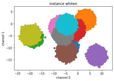
After instance whitening, each instance is circular, but the global covariance across the batch remains.

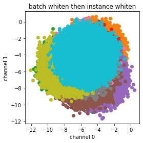
Batch whitening then instance whitening

What happens if we chain the whitening operations? First I’ll try batch -> instance. The data is all scaled down and rotated, then each local distribution is spherized.

_, ax = feature_scatter(instance_whiten(batch_whiten(activations)), nrows=1, ncols=1)
ax[0,0].set(title='batch whiten then instance whiten');

Instance whitening then batch whitening

Next I’ll try instance -> batch whitening.

_, ax = feature_scatter(batch_whiten(instance_whiten(activations)), nrows=1, ncols=1);
ax[0,0].set(title='instance whiten then batch whiten');

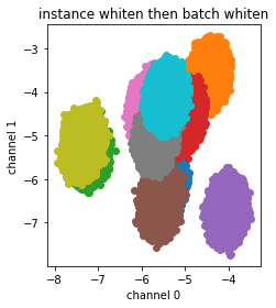
In this case, the local circles are destroyed and turned elliptical again by the global whitening.

Summary

Batch and instance whitening are both useful tools in machine learning. Whether one is better than the other depends on your use-case. There is an interesting paper introducing “Switchable whitening”, proposing to use a weighting of both batch and instance whitening, showing that the relative weighting depends on the task.

Their implementation is different from the cascaded forms of whitening I showed here, which might also be interesting to look into deeper.